Unicycle robot: a discrete-time model with a custom growth bound
| System | 3-D discrete-time, nonlinear |
| Specification | reach-avoid |
| Solver | uniform grid abstraction |
A mobile cart drives in the plane. Its state is the position $(x_1, x_2)$ and the heading $x_3$; the inputs are the linear and angular velocities. Unlike the other examples the model is already discrete in time, so the dynamics are written with Δ rather than ∂ and no sampling step is involved:
\[x^+ = \begin{bmatrix} x_1 + u_1 \cos(x_3) \\ x_2 + u_1 \sin(x_3) \\ x_3 + u_2 \end{bmatrix}.\]
The cart must reach a reference position while staying inside $\{x_1^2 - x_2^2 \le 4,\; 4x_2^2 - x_1^2 \le 16\}$. That region is not a box, so its complement is covered by rectangles and declared as obstacles.
Adapted from the numerical experiments of (Azaki et al., 2022; Sec. 5).
using StaticArrays, JuMP, Plots
using Symbolics, MathOptSymbolicAD

using Dionysos
const DI = Dionysos
const UT = DI.Utils
const ST = DI.System
const MP = DI.Mapping;
The model
hx = 0.1
x_low = [-3.5, -2.6, -pi]
x_upp = -x_low

model = Model(Dionysos.Optimizer);
@variable(model, x_low[i] <= x[i = 1:3] <= x_upp[i])
@variable(model, -1 <= u[1:2] <= 1);
Δ marks a discrete-time model. The modulo $2\pi$ on the heading is left out: Dionysos can treat a coordinate as periodic, but this example does not need it.
@constraint(model, Δ(x[1]) == x[1] + u[1] * cos(x[3]))
@constraint(model, Δ(x[2]) == x[2] + u[1] * sin(x[3]))
@constraint(model, Δ(x[3]) == x[3] + u[2]);

x_initial = [1.0, -1.7, 0.0]
x_target = [sqrt(32) / 3, sqrt(20) / 3, -pi]

@constraint(model, start(x[1]) in MOI.Interval(x_initial[1] - hx, x_initial[1] + hx))
@constraint(model, start(x[2]) in MOI.Interval(x_initial[2] - hx, x_initial[2] + hx))
@constraint(model, start(x[3]) in MOI.Interval(x_initial[3] - hx, x_initial[3] + hx))

@constraint(model, final(x[1]) in MOI.Interval(x_target[1] - hx, x_target[1] + hx))
@constraint(model, final(x[2]) in MOI.Interval(x_target[2] - hx, x_target[2] + hx))
@constraint(model, final(x[3]) in MOI.Interval{Float64}(-pi, pi));
The admissible region is described by two quadratic inequalities. ∉ takes boxes and bounded LazySets, not arbitrary sublevel sets, so the forbidden region is rasterised on a grid and covered by maximal horizontal rectangles.
function extract_rectangles(matrix)
    isempty(matrix) && return []
    n, m = size(matrix)
    tlx, tly, brx, bry = Int[], Int[], Int[], Int[]
    for i in 1:n
        j = 1
        while j <= m
            if matrix[i, j] == 1
                j += 1
                continue
            end
            push!(tlx, j)
            push!(tly, i)
            while j <= m && matrix[i, j] == 0
                j += 1
            end
            push!(brx, j - 1)
            push!(bry, i)
        end
    end
    return zip(tlx, tly, brx, bry)
end

function get_obstacles(lb, ub, h)
    x1 = range(lb[1]; stop = ub[1], step = h)
    x2 = range(lb[2]; stop = ub[2], step = h)
    X1 = x1' .* ones(length(x2))
    X2 = ones(length(x1))' .* x2
    admissible = ((X1 .^ 2 .- X2 .^ 2) .<= 4) .& ((4 .* X2 .^ 2 .- X1 .^ 2) .<= 16)
    return [
        MOI.HyperRectangle([x1[a], x2[b]], [x1[c], x2[d]]) for
        (a, b, c, d) in extract_rectangles(admissible)
    ]
end

for obstacle in get_obstacles(x_low, x_upp, hx)
    @constraint(model, x[1:2] ∉ obstacle)
end
The abstraction
This example supplies a growth bound map directly rather than a Jacobian bound: given a cell radius r and an input, it returns the radius of a box containing the successors. It is a radius, so it must be nonnegative for every admissible input — hence abs(u[1]).
function growth_bound(r, u)
    β = abs(u[1]) * r[3]
    return SVector{3}(β, β, 0.0)
end

set_attribute(model, "growthbound_map", growth_bound)
set_attribute(
    model,
    "state_grid",
    MP.GridFree(SVector(0.0, 0.0, 0.0), SVector(hx, hx, 0.2)),
)
set_attribute(model, "input_grid", MP.GridFree(SVector(1.1, 0.0), SVector(0.3, 0.3)))
set_attribute(model, "print_level", 0);
Solving
optimize!(model);┌ Warning: Some transitions jump 11.0 cells per step while the state domain has holes: the trajectory between two samples may cross an excluded region unchecked. Consider a time step below `MP.intersample_safe_time_step(state_grid, velocity_bound)` (one cell per axis per step) so that inter-sample trajectories stay in certified cells.
└ @ Dionysos.Optim.Abstraction.UniformGridAbstraction ~/.julia/packages/Dionysos/tsG4k/src/optim/continuous_systems/UniformGridAbstraction/alternating_simulation_problem.jl:795
┌ Warning: The `state_cost` is not yet fully implemented
└ @ Dionysos.Optim.Abstraction.UniformGridAbstraction ~/.julia/packages/Dionysos/tsG4k/src/optim/continuous_systems/UniformGridAbstraction/optimal_control_problem.jl:167Results
termination_status(model)OPTIMAL::TerminationStatusCode = 1abstract_system = get_attribute(model, "abstract_system");
abstract_value_function = get_attribute(model, "abstract_value_function");
concrete_problem = get_attribute(model, "concrete_problem");Closed loop
trajectory = Dionysos.simulate(model, SVector(x_initial...); nsteps = 100);Visualisation
The specification sets are 3-D, so they are projected onto the plotted plane explicitly: plot!(concrete_problem) would hand LazySets a 3-D polytope, which needs a convex-hull backend. Everything else already defaults to dims = [1, 2].
fig = plot(; aspect_ratio = :equal)
plot!(concrete_problem.system.X; color = :grey, opacity = 0.5, label = "")
plot!(abstract_system; value_function = abstract_value_function)
plot!(
    UT.project_set(concrete_problem.initial_set, [1, 2]);
    color = :green,
    opacity = 0.5,
    label = "Initial set",
)
plot!(
    UT.project_set(concrete_problem.target_set, [1, 2]);
    color = :red,
    opacity = 0.5,
    label = "Target set",
)
plot!(trajectory; ms = 2.0, lw = 2, color = :blue)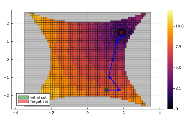
The same run as an animation: the cart and its heading on the left, the state and input channels on the right.
include(
    joinpath(
        dirname(dirname(pathof(Dionysos))),
        "problems",
        "UnicycleRobot",
        "unicycle_robot.jl",
    ),
);

anim = Dionysos.animate_trajectory_dashboard(
    UnicycleRobot.system_plot!(;
        xlims = (x_low[1], x_upp[1]),
        ylims = (x_low[2], x_upp[2]),
    ),
    trajectory;
    xdims = (1, 2),
    udims = (1, 2),
    Δt = 1.0,
    xlabel_state = "x₁",
    ylabel_state = "x₂",
    xlabel_input = "step",
);
gif(anim; fps = 8)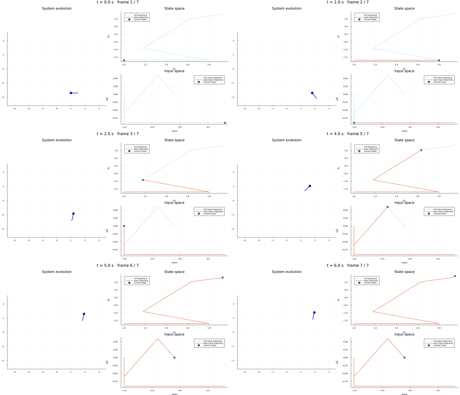
This page was generated using Literate.jl.