Velocity-controlled biped: a certified footstep
The model and its assumptions
The robot is a planar biped: two legs (hip + knee joints each), the stance foot pinned at the origin. The state is the vector of the four joint angles x = (θ₁, θ₂, θ₃, θ₄) (stance hip, stance knee, swing hip, swing knee); every Cartesian quantity follows by forward kinematics. The input is the vector of commanded joint velocities, and the dynamics are the pure integrator
\[\dot{x} = u .\]
This is a deliberate change of abstraction level compared to the 6-D/8-D torque-controlled models of the same robot: instead of certifying the multibody dynamics, we delegate the torque level to the motors' low-level velocity controllers and certify the kinematic layer above them. The assumptions are:
- the low-level controllers track the commanded velocity within the sampling period. A bounded tracking error
εcan later be re-imported as a disturbance: the abstraction then stops being a bisimulation and becomes an alternating simulation with a quantified margin — still sound, no longer exact; - the motion is quasi-static (balance is not part of the specification) and the stance foot stays pinned.
The payoff: the state dimension halves (angles only — velocities are now inputs) and f(x, u) = x + τ·u is exact.
using StaticArrays
using JuMP
using Symbolics, MathOptSymbolicAD # compile the ∂ dynamics of the front-end
using Dionysos
import LazySets
import Plots

const DI = Dionysos
const MP = DI.Mapping
const ST = DI.SystemDionysos.SystemForward kinematics
Segment lengths follow the canonical robot constants. The swing-foot position is the only map the constraints need; the plotting helper reuses the intermediate joints.
const L1 = 0.20125 # hip → knee
const L2 = 0.172   # knee → foot

function joint_positions(θ::SVector{4})
    knee_s = L2 * SVector(-sin(θ[1] + θ[2]), cos(θ[1] + θ[2]))     # stance knee
    hip = knee_s + L1 * SVector(-sin(θ[1]), cos(θ[1]))
    knee_w = hip + L1 * SVector(sin(θ[3]), -cos(θ[3]))             # swing knee
    foot = knee_w + L2 * SVector(sin(θ[3] + θ[4]), -cos(θ[3] + θ[4]))
    return (; knee_s, hip, knee_w, foot)
end

swing_foot(θ::SVector{4}) = joint_positions(θ).foot
swing_foot (generic function with 1 method)Discretization: an abstraction that is a bisimulation
Pick the input grid so that one sampling period moves the state by a whole number of cells: τ · du = dx. Every admissible input then translates the state grid exactly onto itself, so the reach set of a cell is a cell — no over-approximation, no spurious transition. The abstraction is then a bisimulation of the concrete system rather than merely an alternating simulation, which is what makes the CENTER_SIMULATION approximation mode legitimate here: propagating the cell centre is unsound in general, and exact under this choice of grids.
("Commensurable grids" below is the ordinary mathematical sense of the word — the ratio dx / (τ·du) is an integer. The term of art is the result: bisimulation.)
dx, τ = 0.1, 0.1
du = dx / τ                       # one speed notch; u ∈ {-du, 0, du} per joint
state_grid = MP.GridFree(SVector(0.0, 0.0, 0.0, 0.0), SVector(dx, dx, dx, dx))
input_grid = MP.GridFree(SVector(0.0, 0.0, 0.0, 0.0), SVector(du, du, du, du))
Dionysos.Mapping.GridFree{4, Float64}([0.0, 0.0, 0.0, 0.0], [1.0, 1.0, 1.0, 1.0])Physical constraints, pulled back to joint space
The constraints are not on the state: they are on the swing foot, a nonlinear image of it,
\[g : \mathbb{R}^4 \to \mathbb{R}^2, \qquad g(θ) = \text{swing foot position}.\]
The abstraction, however, reasons about cells. So each constraint must be pulled back: a grid cell is dropped from the state space when some configuration inside it could violate the constraint. Testing the cell centre alone would be unsound — the obstacle preimage is a thin shell that crosses cells without containing their centres, and a trajectory would then walk straight through it.
The Lipschitz bound
What makes a centre test sound is a bound on how far g can move inside one cell. For a cell of half-widths h/2 centred at c,
\[\|g(θ) - g(c)\|_\infty \;\le\; \sum_i L_i \, \frac{h_i}{2} \;=:\; \mathrm{dev}, \qquad L_i = \sup \left| \frac{\partial g}{\partial θ_i} \right| .\]
The Lᵢ are read off the kinematic chain, no differentiation required — each joint rotates everything below it, so the foot moves at most the length of that sub-chain per radian:
θ₁(stance hip) rotates both stance segments, leverL1 + L2;θ₂(stance knee) rotates only the stance shank, leverL2;θ₃(swing hip) rotates both swing segments, leverL1 + L2;θ₄(swing knee) rotates only the swing shank, leverL2.
Hence L = (L1+L2, L2, L1+L2, L2), and the whole leg being rigid below each joint, the bound is tight up to the ∞-norm relaxation.
Removing cells soundly
With that bound, two constraints are carved out of the state space:
- the ground,
g(θ)_y ≥ 0— active along the entire swing, since the foot travels at floor level from behind the robot to the foothold. It is a closed contact constraint (the target foothold lies on the floor), so a cell is removed only when every configuration in it is surely below ground,g(c)_y < -\mathrm{dev}. Boundary cells are deliberately kept, accurate to the grid resolution; - a Cartesian obstacle
O— a cell is removed as soon as some configuration in it might reach it:\[\text{remove } C \iff \big( g(c) \oplus [-\mathrm{dev}, \mathrm{dev}]^2 \big) \cap O \neq \emptyset .\]
Contrapositive, which is the certificate: a kept cell satisfiesg(θ) ∉ Ofor everyθin it.
The margin is also an honest feasibility detector. At dx = 0.1 it is dev ≈ 5.5 cm; an obstacle sitting under the swing path then provably disconnects the free space, and no controller exists at this resolution — stepping over one needs a finer grid and a wider joint range (that run is examples/BipedRobot/biped_4d_velocity.jl, ≈ 2.5 M cells). Here the obstacle is placed just behind the start, so the run stays a few seconds; the ground, which is the constraint that actually shapes this motion, is carved all the same.
obstacle =
    LazySets.VPolygon([SVector(-0.39, 0.0), SVector(-0.35, 0.02), SVector(-0.31, 0.0)])

x_bar = 0.6
X_box = LazySets.Hyperrectangle(;
    low = SVector(-x_bar, -x_bar, -x_bar, -x_bar),
    high = SVector(x_bar, x_bar, x_bar, x_bar),
)

grad = SVector(L1 + L2, L2, L1 + L2, L2)
dev = sum(grad .* MP.get_h(state_grid) ./ 2)

# `MP.cells_where` collects grid cells by predicate into a `MP.CellUnion` — a
# cell-aligned set whose discretization is exact, so a hole removes exactly its
# own cells and a target is recovered exactly. `MP.image_blocked_cells(g, L, …)`
# packages this same Lipschitz pullback for any nonlinear image map; it is
# spelled out here to keep every ingredient visible.
removed = MP.cells_where(state_grid, X_box) do pos
    foot = swing_foot(SVector{4}(MP.get_coord_by_pos(state_grid, pos)))
    below_ground = foot[2] < -dev
    hits_obstacle =
        !Dionysos.Utils.is_disjoint(
            LazySets.Hyperrectangle(foot, SVector(dev, dev)),
            obstacle,
        )
    return below_ground || hits_obstacle
end
length(removed)1774Between two samples
Carving certifies the cells; the abstraction only ever checks the state at sampling instants. What forbids the trajectory from cutting a corner between two samples is a second, independent ingredient — and the two together are what make the run sound.
For ẋ = u the inter-sample trajectory is the straight segment joining two consecutive states. Two regimes:
- one cell per axis per step (
τ·|u| ≤ h, the case below): the segment cannot leave the union of the source and target cells, both certified, so nothing more is needed.MP.intersample_safe_time_stepreturns the largestτrespecting this; - larger inputs, which move several cells per step: the segment then crosses intermediate cells that no endpoint check ever looks at.
MP.cells_on_segmentenumerates exactly those crossed cells, andMP.swept_input_filterkeeps a transition only when all of them are admissible. That is what lets the input alphabet carry several speeds without giving up soundness.
Bounding τ by the obstacle width instead — the natural first idea — is not sound: it prevents stepping fully over an obstacle, yet still allows grazing a corner between two free endpoints.
MP.cells_on_segment(
    state_grid,
    SVector(0.0, 0.0, 0.0, 0.0),
    SVector(0.2, 0.1, 0.0, 0.0), # a two-cell step along θ₁, one along θ₂
)
4-element Vector{NTuple{4, Int64}}:
(0, 0, 0, 0)
(1, 0, 0, 0)
(1, 1, 0, 0)
(2, 1, 0, 0)The objective: place the swing foot on the target foothold
The target is the set of configurations whose swing foot lies on the foothold — a 2-D manifold in the 4-D joint space. Sweeping the stance angles and solving the swing leg's two-link inverse kinematics (elbow-down) enumerates it; quantizing to grid cells (deduplicated) gives the target set.
foothold = SVector(0.2, 0.0)

target_cells = Set{NTuple{4, Int}}()
for θ1 in range(-x_bar, x_bar; step = dx / 3), θ2 in range(-x_bar, x_bar; step = dx / 3)
    hip = joint_positions(SVector(θ1, θ2, 0.0, 0.0)).hip
    d = foothold - hip
    c4 = (d[1]^2 + d[2]^2 - L1^2 - L2^2) / (2 * L1 * L2)
    -1.0 <= c4 <= 1.0 || continue
    θ4 = -acos(c4)
    θ3 = atan(d[1], -d[2]) - atan(L2 * sin(θ4), L1 + L2 * cos(θ4))
    θ = SVector(θ1, θ2, θ3, θ4)
    all(abs.(θ) .<= x_bar) || continue
    push!(target_cells, MP.get_pos_by_coord(state_grid, θ))
end
target_set = MP.CellUnion(state_grid, target_cells)
length(target_cells)76The JuMP model
Everything above becomes a few declarative lines: variables with bounds, the integrator dynamics through ∂, the carved region through ∉, the target through Final, and the discretization through solver attributes.
x0 = SVector(0.2, 0.0, -0.2, 0.0)

model = Model(Dionysos.Optimizer)
@variable(model, -x_bar <= x[i = 1:4] <= x_bar, start = x0[i])
@variable(model, -du <= u[1:4] <= du)
@constraint(model, [i = 1:4], ∂(x[i]) == u[i])
@constraint(model, x ∉ removed)
@constraint(model, x in Final(target_set))

set_attribute(model, "time_step", τ)
set_attribute(model, "state_grid", state_grid)
set_attribute(model, "input_grid", input_grid)
set_attribute(
    model,
    "approx_mode",
    DI.Optim.Abstraction.UniformGridAbstraction.CENTER_SIMULATION,
)

optimize!(model)
get_attribute(model, "success")trueClosed loop of this unconstrained controller, to compare against the slew-rate-limited one below:
controller_free = get_attribute(model, "concrete_controller")
discrete_time_system = get_attribute(model, "discrete_time_system")

reached(xk) = xk ∈ target_set
traj_free = ST.get_closed_loop_trajectory(
    discrete_time_system,
    controller_free,
    x0,
    100;
    stopping = reached,
)
xs_free = collect(ST.states(traj_free))
(length(xs_free) - 1, reached(xs_free[end]))
(5, true)The acceleration constraint
Because the inputs are velocities, bounding the difference between consecutive inputs is an acceleration (slew-rate) limit — precisely what makes the command trackable by the motors, closing the loop with assumption 1. The value function of this constrained synthesis lives on (state, input) pairs (the classical turn-restricted shortest path), and the controller is dynamic: its memory is the previously played input. (OPDS.BoundedInputVariation.) Here: at most one speed notch of change per joint per step, starting from and ramping down to rest.
rest = SVector(0.0, 0.0, 0.0, 0.0)
slew = DI.Optim.DiscreteSystems.BoundedInputVariation(
    (u1, u2) -> maximum(abs.(u1 - u2)),
    du;
    target_input = rest,
    initial_input = rest,
)
set_attribute(model, "bounded_input_variation", slew)
optimize!(model)
get_attribute(model, "success")trueClosed loop of the constrained controller — a few steps longer than the unconstrained one: the difference is the acceleration ramps.
controller = get_attribute(model, "concrete_controller")
traj = ST.get_closed_loop_trajectory(
    discrete_time_system,
    controller,
    x0,
    100;
    stopping = reached,
)
xs = collect(ST.states(traj))
us = collect(ST.inputs(traj))
(length(xs) - 1, reached(xs[end]))
(5, true)maximum(maximum(abs.(us[k + 1] - us[k])) for k in 1:(length(us) - 1))1.0The measured maximum input variation sits exactly at the bound: the constraint is active and satisfied along the whole run.
Visualizing the footstep
function draw_robot!(fig, θ::SVector{4})
    p = joint_positions(θ)
    Plots.plot!(
        fig,
        [0.0, p.knee_s[1], p.hip[1]],
        [0.0, p.knee_s[2], p.hip[2]];
        lw = 4,
        marker = :circle,
        color = :steelblue,
        label = "",
    )
    Plots.plot!(
        fig,
        [p.hip[1], p.knee_w[1], p.foot[1]],
        [p.hip[2], p.knee_w[2], p.foot[2]];
        lw = 4,
        marker = :circle,
        color = :indianred,
        label = "",
    )
    return fig
end

fig = Plots.plot(; aspect_ratio = :equal, legend = false, xlims = (-0.6, 0.6))
Plots.plot!(fig, [-0.6, 0.6], [0.0, 0.0]; color = :black, lw = 1, label = "")
Plots.plot!(fig, obstacle; color = :black, alpha = 0.8, label = "")
Plots.scatter!(fig, [foothold[1]], [foothold[2]]; marker = :xcross, color = :green)
for (k, xk) in enumerate(xs)
    (k % 4 == 1 || k == length(xs)) && draw_robot!(fig, xk)
end
fig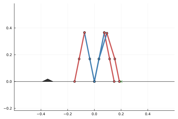
The blue stance leg stays planted, the red swing leg travels from behind to the green foothold.
The same trajectory as an animation, with the state and input panels beside it — the swing angles (θ₃, θ₄) and the velocities commanded to them:
function system_plot!(fig, xk, uk)
    Plots.plot!(fig, [-0.6, 0.6], [0.0, 0.0]; color = :black, lw = 1, label = "")
    Plots.plot!(fig, obstacle; color = :black, alpha = 0.8, label = "")
    Plots.scatter!(fig, [foothold[1]], [foothold[2]]; marker = :xcross, color = :green)
    draw_robot!(fig, SVector{4}(xk))
    Plots.plot!(fig; xlims = (-0.6, 0.6), ylims = (-0.05, 0.5))
    return fig
end

anim = DI.animate_trajectory_dashboard(
    system_plot!,
    traj;
    Δt = τ,
    xdims = (3, 4),
    udims = (3, 4),
    xlabel_state = "θ3 (swing hip)",
    ylabel_state = "θ4 (swing knee)",
    xlabel_input = "u3 (swing hip)",
    ylabel_input = "u4 (swing knee)",
    title = "Certified footstep",
)
Plots.gif(anim; fps = 8)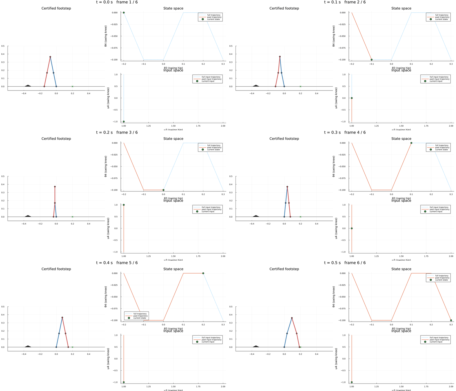
What is certified, and what is not
Certified: the closed-loop joint trajectory reaches the target foothold manifold, never drives the swing foot into the obstacle or below the ground — at sampling instants and in between — and respects the input slew-rate limit with rest-to-rest ramps.
Assumed: the low-level velocity tracking (assumption 1) and the quasi-static regime (assumption 2). Quantifying the tracking error and re-importing it as a bounded disturbance is the natural next step — the growth-bound machinery accepts it directly, at the price of an abstraction that is no longer a bisimulation but remains sound.
This page was generated using Literate.jl.